2024 NFL Week 2 DFS Breakdown: Winning Lineups and Strategies
by Ryan Baker · Published · Updated
One effective way to succeed at something is by studying past winners. In this case, we’re going to look at the 2024 winners of DraftKings’ flagship contest, the Milly Maker (NFL $3.5M Fantasy Football Millionaire).
The Milly Maker is a Mass Multi-Entry (MME) contest, allowing participants to enter up to 150 lineups. With over 200,000 entries, it attracts both beginners and seasoned professionals, making it highly competitive. Although we aren’t evaluating FanDuel contests this year, many of the same principles apply, so this information can still be valuable for those playing on that platform.
It’s important to remember that just because something worked in one instance doesn’t mean it will work again. That’s where the science of probability comes into play. While analyzing past data can help us identify trends and strategies, outcomes in contests like these are influenced by numerous variables, making history a helpful guide but not a guaranteed predictor.
By studying the winners, we can uncover patterns, but we must also acknowledge that unpredictability is common in such large contests. In this article, I’ll break down what I’m looking at and in future weeks, I’ll more or less just share the data.
To start off, I’ve analyzed the top lineups from both Week 1 and Week 2, breaking them down into common strategies to see what worked for the winners. My focus is on understanding the type or roster construction they used, which positions were popular in the flex spot, how much of their salary cap they spent, and the total ownership percentage of their rosters.
For those short on time, here is the TLDR version:
So what happened in the first two weeks with the winning lineups?
- RBs have been a popular choice in the flex spot.
- Max out your salary whenever possible.
- The top lineups hover around 100% total roster ownership.
- Current PTP value is 4.15x (down from last year)
- Differentiating yourself from the field is key in MME tournaments.
- You can play some chalk players, but in moderation.
- Save money at QB and TE, spend big at RB and WR.
- No one has all the answers—adapt as you go.
First, let’s look at the two winning lineups.
Here is Week 1’s winner: sidi1979
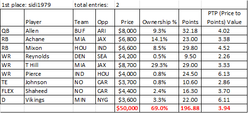
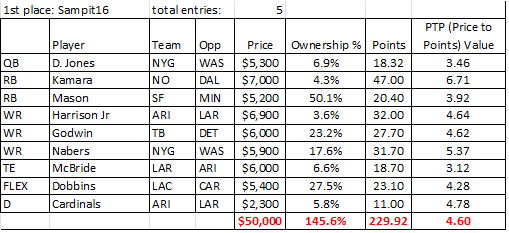
Here is Week 2’s winner: Sampit16
ROSTER CONSTRUCTION
I analyzed the top 10 lineups from Week 1 and Week 2, for a total of 20 lineups, and two things stood out compared to last year.
- Scoring is down. The winning week 1 lineup only scored 196.88 points. Typically the winning lineup scores over 220 points. For context, last year’s Week 1 winner scored 233.24 points.
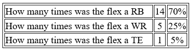
- The dominance of running backs (RB) in the flex position, with 70% of the top lineups (18 out of 20) using an RB in the flex 25% of the time, and Tight End (TE) 5% of the time. Historically, this RB trend is unlikely to continue at such a high rate.
Due to time constraints, I wasn’t able to evaluate every week’s winning lineup last year, so I won’t throw out half-baked data (he goes on to throw out half-baked data anyway). However, I can tell you that in the 32 lineups I did evaluate, WRs appeared in the flex over 60% of the time, RBs around 35%, and TEs roughly 5%.
The key takeaway is that we should expect more (WR) in the flex among future winning lineups compared to the current trend. If you like to follow trends, you should probably play a RB in your flex. If you like to buck trends before they buck you, you should play a WR in your flex.
Another interesting observation from these 20 lineups is that in two instances, a winning lineup had a defense (D) starting against offensive players from the opposing team. Let’s call the OD for Oppositional Defense. This is generally considered a faux pas among experts, who advise against playing a defense against any of your offensive players.
While avoiding an OD is usually sound advice, there are situations where it can pay off, albeit a long shot. Salary savings is the most common way it could pay off. Less likely is if the defense scores touchdowns through turnovers or returns, that would force the opposing offense to stay aggressive. While predicting defensive touchdowns isn’t something we’re recommending to do, it’s worth noting that sometimes the ‘rules’ of roster construction are flexible.
STACKING
The most common stack we observed was the QB paired with one WR, occurring in 45% of the 20 lineups we evaluated.
The defense was paired with another player from their team 40% of the time, whether a QB, RB, WR, or TE. I haven’t traditionally focused on this strategy, partly due to my struggles with picking the right defense in a given week, but it’s an area I’m working to improve.
The data reinforced what we already know: stacking is crucial. While having a “naked” QB (no teammate tied to the QB) can win you money, incorporating other stacks in your lineup is essential. Overall though, make it easy on yourself and stack your QB!
RAW STATISTICS FROM FIRST TWO WEEKS
Given the small sample size, these numbers we’re about to show will adjust every week and start to paint a clearer picture. There will be some outliers and perhaps you’ll be the one to make a difference—maybe your lineup will be the first to stack a QB with their RB and take it all down. Just because 0 have hit in the top lineups definitely does not mean it won’t. I expect all of the stacking options below to hit this year.
Here are the raw statistics out of 20 lineups:
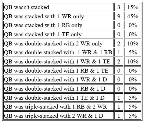
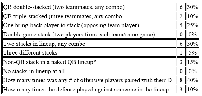
*Note: Every lineup that had a naked QB all had a stack somewhere else in their lineup. 3 teams rolled with a naked QB and all 3 had stacks somewhere else in their lineup.
SALARY
Now that we’ve covered the positions, let’s discuss salary. Let’s KISS (Keep it Simple Stupid): spend as much as possible!
I looked at the top 5 lineups from the first two weeks and the average salary spent on winning lineups for the first two weeks was $49,820, which is 99.64% of the total. Both Week 1 and Week 2’s winning lineups used the full $50,000.
In terms of where to allocate your money, every slate is different. Sometimes there are high-priced QBs on the slate, sometimes there aren’t. Sometimes there are high-priced TEs, sometimes there aren’t. You get the idea. While it’s challenging to pinpoint exact spending strategies due to these variations, we can use data to offer some guidance.
Here’s how the top 10 teams allocated their money in the first two weeks, on average:
QB: $5,820
RBs: $6,215 per RB
WRs: $6,110 per WR
TEs: $4,450
Flex**: $5,560
D: $3,230
**Note, the position used in the flex isn’t accounted for in the averages for individual positions.
As I mentioned earlier, take these numbers with a grain of salt. This is a small sample size. In week 1, the average amount spent on the defense was $3,560, which is pretty high, and in week 2, it was $2,900. Week 3 could be much lower, who knows.
From these averages, it’s clear that saving money at QB and TE while focusing on RB and WR is often effective. Top-tier QBs and TEs like Mahomes and Kelce can be game-changers, but their high cost means they need to perform exceptionally to justify the investment. While it’s possible for them to deliver big returns, it’s good to not bank on the highest-priced QBs and TEs every week.
OWNERSHIP
Different platforms use varying methods, and while technology is improving, the projections can still be hit or miss. Last year, I subscribed to several services, but their projections varied and often weren’t as accurate as I’d like. It doesn’t mean they aren’t helpful but you need to limit your expectations when seeing projections.
In any contest, certain players are bound to be more popular plays, often referred to as “chalk” players. While there’s no exact percentage that defines a chalk player, it typically refers to any player with ownership above 20%-ish.
High-ownership players are generally considered safer because of their perceived value. However, success in Mass Multi-Entry (MME) tournaments often comes from striking a balance between popular, chalk plays and lower-owned players to make your lineup stand out. Differentiation from the crowd is key to winning.
There are times when the chalk play is simply too good to pass up. Take Week 2, for example: it was clear that Jordan Mason, stepping in as the 49ers’ starting running back, was an excellent value. His salary on DraftKings hadn’t adjusted to reflect his new role, making him a bargain compared to others in his price range. While that doesn’t mean you should include him in every lineup, it does mean having exposure to him in some lineups is wise.
On the flip side, sometimes avoiding the chalk gives you leverage against the field, so it’s a case-by-case decision. Recognizing when to play the chalk and when to pivot can make the difference between a winning lineup and one that fades into the background.
In years past, I’ve seen lineups win with a ton of highly-owned players, and others with an incredible mix of low-owned players. We can use this year’s data to reference to try and find a range you can shoot for.
Out of the 10 lineups I evaluated, the lowest total ownership was 48.6%, which came from the 5th-place team in Week 2. This is impressive and was largely due to a very low-owned Seattle stack. Interestingly, their highest-owned players underperformed, meaning a slight adjustment could have put this team in a position to take down the entire contest.
The highest total ownership for a roster was 145.6%, which won week 2. They had Mason who came in at 50.1% owned, Dobbins at 27.5%, and Godwin at 23.2%. Chalk can win. They also had a low-owned Harrison Jr (3.6%) and Kamara (4.3%).
The average ownership across the top 10 lineups was 100.74%, which aligns with my target range of 90% – 120%. Anything higher means you’re probably not being unique enough, while anything lower might be “too cute.” It’s similar to straying too far from ADP in best ball drafts—essentially betting that the field doesn’t know what it’s doing. The reality? The field misses more than you’d expect, and chalk can and does fail. That said, going under 90% ownership is a challenge, so if you’re going for it, more power to you!
As mentioned earlier, scoring is down, so that makes sense that the player’s value is down a bit too. What I call “value”, I really mean the price to points (PTP) value. The PTP value shows how many points you need from a player based on their salary to win. To calculate it, you divide a player’s points by their adjusted salary (which is their salary divided by 1,000). For example, if a player costs $5,000, the adjusted salary is 5.0. If the target PTP value is 3.53, you multiply the adjusted salary by 3.53 to find the points you need. So, for a $5,000 player, you’d want 17.65 points (5 x 3.53) to hit your target value.
Right now, the PTP average for top lineups is 4.15x, but last year, it was around 4.4x through the first two weeks and 4.82x through eight weeks. So, I expect an adjustment soon, unless the hype around two high safety defenses really sticks. Regardless, you’ll still want to aim for players with the best PTP on any slate to maximize value.
NUMBER OF ENTRIES
What I always find fascinating is how many lineups the winners enter into the tournament. In Week 1, the top 5 lineups averaged just 2.2 entries per person. Week 1 is also the only week where the entry fee is $5, leading to more entries overall. Still, it’s impressive that the top 5 players didn’t rely on mass-entering. In Week 2, we saw a few people who did mass-enter, with the average entries for the top 5 players jumping to 76.4. Despite that, the Milly winner in Week 1 only entered twice, and the winner in Week 2 entered just five times. So there’s hope for everyone!
That wraps up our Week 2 analysis of winning lineups! Keep in mind that these insights are intended to guide your strategy, not act as strict guidelines.